The authors of this paper explored whether the new questions together could predict trust levels, considering them as a potential scale. We wanted to understand if the scale was a reasonable predictor of trust over and above the demographic characteristics captured in the survey.
An exploratory factor analysis indicated a one factor structure, with one dimension having an eigenvalue above one, as shown below in the scree plot. The items together made a scale with a Cronbach’s alpha of 0.95 for both the pilot (excellent internal consistency, as any value above .70 is acceptable, and .80 is good). Removing any of the items reduced the alpha level, so all were retained for further analysis.
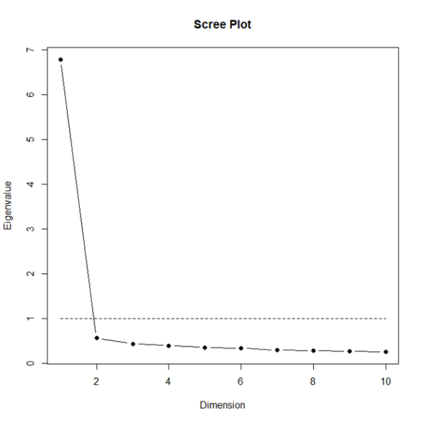
Figure 1 Scree plot on trust drivers for pilot data
Following the factor analysis for the question on drivers and trust, an average score across the ten items in the question was calculated as the single measure of drivers of trust to be used in further analysis.
The independent variable, the new drivers scale, had a mean of 3.6 with a standard deviation of 0.8, and a range from 1 to 5 (covering all points on the response scale). The dependent variable, trust in the Public Service, had a mean score of 3.7 with a standard deviation of 0.9, and had a range from 1 to 5.
There was a strong and statistically significant correlation between the average score across the drivers question and the dependent variable of trust in the Public Service.
To examine the relationship between the average drivers of trust score and the trust in Public Service in more detail, a hierarchical linear regression was carried out using R. The first model aimed to see how the demographic variables affected the dependent variable, while the second model checked to see if the average drivers score (independent variable) had an effect once those demographic variables had been taken into account.
We tested the following models for their impact on trust in the Public Service:
Model 1: Gender + Age Group + Household Income[1] + Disability + Highest qualification + Ethnicity groupings
Model 2: Gender + Age Group + Household Income + Disability + Highest qualification + Ethnicity groupings + Average drivers score
Table 2 Hierarchical Linear Regression models
-
Model One
Model One
Factor level
b[2]
(Intercept)[3]
3.57**
Gender
Female
-0.09*
Another gender
0.24
Age Group
25-34 years
-0.00
35-44 years
-0.03
45-54 years
-0.14
55-64 years
-0.15
65-74 years
-0.02
75+ years
0.12
Household Income
$50,001-$100,000
0.12*
>$100,0000
0.09
Disability
No
0.13*
Education
School level qualification
0.15
Post-school certificate
0.15
Degree or postgraduate
0.14
Other
1.28
Ethnicity
NZ European
-0.06
Māori
-0.04
Pacific Peoples
0.07
Asian/Indian
0.17
MELAA
-0.09
Other
0.04
Model One[4] R²= .027**
-
Model Two
Model Two
(Intercept)
0.88**
Gender
Female
-0.06
Another gender
-0.11
Age Group
25-34 years
0.05
35-44 years
-0.03
45-54 years
-0.05
55-64 years
0.01
65-74 years
0.08
75+ years
0.12
Household Income
$50,001-$100,000
0.08
>$100,0000
0.06
Disability
No
0.13**
Education
School level qualification
0.04
Post-school certificate
0.10
Degree or postgraduate
0.08
Other
1.15
Ethnicity
NZ European
-0.03
Māori
-0.03
Pacific Peoples
-0.01
Asian/Indian
0.07
MELAA
0.00
Other
0.00
Drivers
Row mean
0.74**
Model Two R²= .420**
Δ[5] R² = .393**
F = 1209
Pr(>F) < 2.2e-16 ***
*p<.05 **p<.01 *** p<.001
The output of these regressions can be found in the Appendix of this report. The main findings from the regressions were that:
- The average driver of trust score had a statistically significant coefficient even after including the demographic variables in the model.
- Adding the average driver of trust score into the model increased the explanatory power of the model significantly.
- Disability was the only demographic variable that also had a significant coefficient in the final model.
[1] Household income was tested both as collected and aggregated into three similarly sized group to reduce the number of levels being included in the model. The coefficients for the aggregated version is presented here.
[2] Beta (noted as b) estimates the change in the dependent variable (in this case trust in the Public Service) when the independent variable increases one unit, while holding all of the other independent variables constant (i.e., controlling for all of the other demographic factors).
[3] Baseline factor levels for the models are: Gender – Male, Age Group – 16-24 years, Household income (aggregated) - <$50,000, Disability – Yes, Education – No qualification, all ethnicities listed – No.
[4] R2 statistic tells you how much variation in the dependent variable (in this case, trust in the Public Service) the independent variables collectively explain.
[5] Change in R2 tells you how much better the second model is in predicting your dependent variable. In this case, adding the drivers variables increases the predictive ability of the model, even when controlling for demographic characteristics.